
Struggling to find data manually in long spreadsheets? How to Use VLOOKUP in Excel is your shortcut to instant lookup success. In this beginner friendly tutorial you will learn what VLOOKUP does, how its four parameters work, and how to build a reliable lookup formula without endless scrolling. Follow along with a clear example: fetching a product price using a product code. We will guide you through writing the formula manually and using Excel’s FX wizard, plus cover common mistakes and best practices. A free practice file is included so you can follow every step on your own sheet. By the end you will master the basics of VLOOKUP, know how to avoid errors, and be ready to move on to more advanced lookup tools like XLOOKUP or INDEX MATCH. Let’s dive in and make your Excel data lookup smooth and effortless!
Explore more tutorials at Spreadsheet Success or return to the homepage for more resources.
Why You Need VLOOKUP
VLOOKUP saves time by instantly finding matching data. No more scrolling through thousands of rows manually. With large datasets, scrolling is inefficient and error prone. VLOOKUP automates the lookup process.
Understanding VLOOKUP Syntax
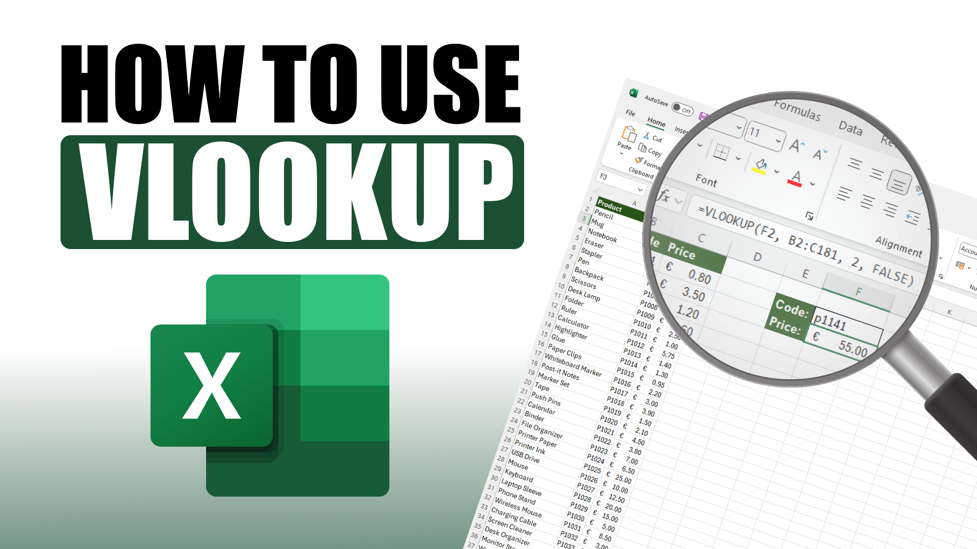
Let’s break down the VLOOKUP function into its four essential parts:
- lookup_value: the value you want to find. Usually a cell reference like F2.
- table_array: the range of cells that contains the data. For example, B2:C181.
- col_index_num: the column number within the table array to return data from.
- range_lookup: enter FALSE for exact matches and TRUE for approximate (we use FALSE).
Use absolute references like $B$2:$C$181 when copying formulas to prevent errors.
Step by Step VLOOKUP Tutorial
Follow along with this practical example:
- Setup: Your sheet has product codes and prices in a table.
- Formula: In your target cell, enter:
=VLOOKUP(F2,B2:C181,2,FALSE)This looks up the code in F2, searches column B, and returns the matching price from column C. - FX Wizard: Click the “fx” button beside the formula bar. Choose VLOOKUP, and fill in the same values. This interface helps if you are unsure about syntax.
Double-check your result by comparing with the original table entry.
Common Mistakes and How to Fix Them
- #N/A error: Occurs if the value is not found. Make sure the value exists and spelling matches.
- #REF! error: Happens if the column index is out of range. Check col_index_num.
- Mixed data types: Numbers stored as text can break lookup. Use
VALUE()or clean data.
Pro tip: Always use FALSE to ensure exact matches unless you understand approximate logic.
Alternatives: XLOOKUP and INDEX MATCH
VLOOKUP has limitations:
- Cannot look to the left of the lookup column.
- Breaks if columns are inserted between lookup and return columns.
Use XLOOKUP or INDEX MATCH when you need more flexibility.
- XLOOKUP: Works left to right and right to left. Easier syntax.
- INDEX MATCH: A combination of two functions that offer full control.
Still, VLOOKUP is great for simple lookups and is widely supported.
Quick Takeaways
- VLOOKUP is ideal for vertical lookups using a common identifier.
- Use
=VLOOKUP(lookup_value, table_array, col_index_num, FALSE). - Lock your table_array with $ symbols for consistent results.
- Errors like #N/A and #REF! are common and easily fixed.
- Upgrade to XLOOKUP or INDEX MATCH for complex needs.
FAQs
Can VLOOKUP search left?
No. VLOOKUP only searches to the right. Use INDEX MATCH or XLOOKUP if needed.
Why does VLOOKUP give #N/A?
The value is missing or does not exactly match. Check spelling and data type.
What is the difference between TRUE and FALSE in VLOOKUP?
TRUE finds an approximate match. FALSE finds an exact match and is recommended.
Can VLOOKUP pull from another sheet or workbook?
Yes. Reference the sheet or workbook in your table_array.
Should I use XLOOKUP instead?
If using Excel 365 or 2021, XLOOKUP is simpler and more powerful.
Conclusion
VLOOKUP is one of Excel’s most useful tools for quickly finding matching data. Now that you know how to use it step by step, download the practice file above and give it a try. Whether you are managing a product list, inventory, or client database, this formula can save you time and prevent mistakes.
If you found this guide helpful, consider subscribing to the Spreadsheet Success YouTube channel for more clear and practical tutorials. Check out our tutorial library or visit our homepage for more resources.